
5 essential Excel skills for ITAM professionals
 Excel and other spreadsheets are powerful, universally available tools available for manipulating data. As such, they are popular with the IT Asset Management profession – after all, all that we do is founded upon trustworthy data. As an IT Asset Manager, I probably spent more time than was healthy in my spreadsheets and they became highly complex, undocumented, and unwieldy things being used to provide critical data to my stakeholders. Not ideal.
We’ve seen great advances from tool providers in building analytics, dashboards, and report capabilities into their tools but it’s still the case that we’ll all inevitably end up turning to Excel at some point. With that in mind, I asked the community for tips on using Excel for ITAM – what are the key capabilities and functions that we keep coming back to?
This article takes you on a journey through a typical Excel for ITAM use case – gathering source data, manipulating it, querying it, and finally reporting it. We wrap up with a look at some of the new functionality available in Excel – namely Power Query & Power Pivot. Examples are provided in the article and in the attached sample spreadsheet (click to download).
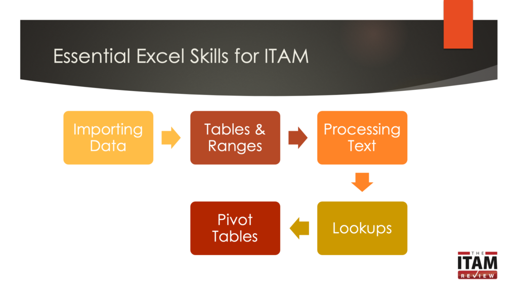
Let’s start with data import tips.
1. Importing data
Often, the reason we’re using Excel is because we’ve got datasets from different sources that we want to combine. Excel’s import functions help here, and mostly you’ll be using CSV (Comma-Separated Values) text imports. These are reliable and relatively quick for static data. There’s very little to go wrong so as long as your source application can export as CSV, you’re good to go.
It is also possible to build live connections to external data using ODBC. You’ll probably need help with this from a database administrator because you’ll need access to the database, but ODBC is reliable, dynamic (real-time), and has fewer manual steps than using text file imports. To build an ODBC connection you’ll need the server name, database name, and the necessary credentials for read access to the database.
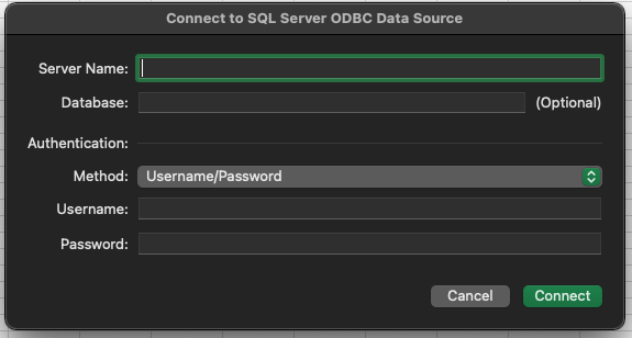
Once connected you use the Data menu to refresh data.
Tip: When using an ODBC connection make sure that your import data destination range is contiguous – place all calculated columns based on the imported data to the right of the import range. This keeps things tidy and easy to manage – when using ODBC connections I apply a colour format to the destination cells as a visual reminder that the data there will be replaced if I refresh the data.
2. Format as Table & Named Ranges
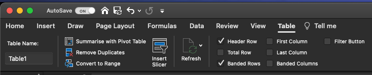
Whenever I import data into Excel, the first thing I do is use the “Format as Table” option on the main ribbon. This helps visually, improves readability, reduces the chance of human error, and also helps with Named Ranges.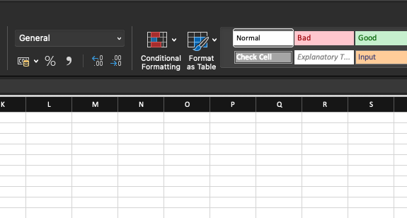
Tip: If you have multiple sheets of data, colour-code the tables on each sheet as a further visual reference. Once again, this will cut down on human error.
With your data formatted as a table the next task is to create Named Ranges.
Why? Named Ranges make it much easier to work with complex formulas and Pivot Tables because you can quickly reference an entire column by name (e.g. Users) rather than use cell references (e.g. A1:A52). To create Named Ranges click the Formulas tab on the ribbon, select all data, & click “Create from Selection”.
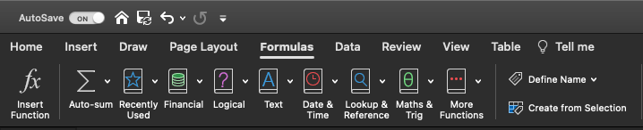
In most cases then untick the “left column” option on the Create Names dialog box.
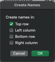
Tip: Before doing this, ensure your column headers are descriptive, unique and short – this helps when using Named Ranges to build formulas.
With your data formatted as a Table and Named Ranges created, you’re ready to get to work. Ideally, get into the habit of doing this every time you import data as it will save you time down the road.
3. Processing Text
Often, data exists in a spreadsheet as text fields, but those aren’t quite in the format we need to run a query or to sort the data. For example, names might be imported as “AJ Witt” whereas we might want to sort by surname. Or a computer name might follow a standard format such as Country/Location/Department/Number (e.g. USNYCFIN0001 is a machine in the New York City office of the Finance Department) but we want to be able to find all computers in New York. This is where string manipulation functions are a great help, particularly the following:
FIND – find the first instance of a character in a string. This is useful for splitting a space-separated string in two.
MID – extract a number of characters from within a string
RIGHT – extract a number of characters from the right of a string
LEFT – extract a number of characters from the left of a string
LEN – find the length of a string – useful for working out the number of characters for MID, RIGHT, & LEFT formulas
VALUE – convert a text value to a number value – needed if you’ve extracted numeric characters from a string and want to use them in calculations.
For more on using these functions including examples please see the attached spreadsheet.
Tip: MID, RIGHT, & LEFT are functions meaning that rather than extracting a fixed number of characters from the string you can calculate that number using another formula – most often LEN.
By looking for patterns in the string you can usually build a parser using a combination of the above functions. With more columns of useful data available your analysis can step up a gear with lookups and other quasi-relational database functions.
4. Lookups, lookups, everywhere
ITAM professionals often need to compare data from different sources and this is where lookups become essential. For example, you may have separate software, hardware, and user inventories which need to be brought together to answer questions such as “Who has used that application on this machine?”. Such questions are best answered via SQL queries to a relational database, but lookups make this possible to do in Excel and the key functions are
- VLOOKUP
- XLOOKUP
- INDEX
- MATCH
Of these, I preferred to use a combination of INDEX & MATCH for most tasks, but VLOOKUP is probably better known, and XLOOKUP is the lookup function you’ve been, um, looking for all these years. In fact, I’d argue it’s the best reason for upgrading to a new version of Excel since the 65,536-row limit was removed by Excel 2007’s introduction of the XLSX file format.
What makes XLOOKUP so great?
Fundamentally, it makes VLOOKUP dynamic and therefore able to cope with sheet design changes such as columns being added. You can also find data in any corresponding column, not just the ones to the right of the lookup target. Rather than say “give me the matching data from the fifth column” it instead says: “give me the matching data from the column I’ve defined”.
The most important change it brings is that by using a column array rather than a specific numbered column, formulas will be automatically updated when the worksheet design changes, and you can look up any column in the source array. This makes lookups truly robust, reduces the risk of error, and in general makes them fit for purpose.
If it’s available to you (you must be an Office 365 subscriber in the Monthly or Semi-Annual channel), it will save you hours, simplify queries, and make your job easier. It does everything VLOOKUP does and more. For those of you unwilling to make the change, don’t worry, as VLOOKUP is still supported, and I’d imagine will be in the product for many years to come.
But what’s the solution to VLOOKUP’s limitations if you don’t have Office 365? Index & Match to the rescue.
Index & Match
Combining the Index & Match functions was the smart way to overcome VLOOKUP’s limitations until XLOOKUP arrived. These two functions enable two-way lookups (combined vertical and horizontal lookups), lookups based on multiple criteria, and case-sensitive searches.
My common use case for Index & Match is to join tables of data together in the same way as you would use JOIN in a SQL query. This is particularly useful for preparing data for use in a Pivot Table. For example, imagine you have a Users table which contains personal data such as employment status, department, location, and so on. You also have a Computers table which contains hardware information and the username of the last user. You can use MATCH to lookup the username in one table and use the result of that formula to pull in data from the other. If there is a column in both tables that’s (ideally) a unique match you can use Index & Match to combine data from both tables.
For examples of how to use Index & Match see the attached workbook.
Note: Office 365 users also have the option to use the new XMATCH function but unlike XLOOKUP it doesn’t really improve the original MATCH function or provide a compelling reason to use it.
5. Pivot Tables
The final tool in the Excel toolbox for ITAM pros is the Pivot Table. Pivot Tables are used to summarise complex data. Their primary use case for ITAM is reporting and forecasting. For example, if your table has a list of computers by department you can automatically build a Pivot table that counts the number of computers in each department. If the table also has office location data in it, you can build a pivot counting computers by location and department. Fold in user data to that and you can even identify how many computers are being used by permanent, contract, and temporary employees.
Pivot tables are now much easier to build and experiment with than they were in earlier versions of Excel. To create one, select any cell in your table (remember, you formatted your spreadsheet as a table after importing it) and click “Summarise with Pivot Table”
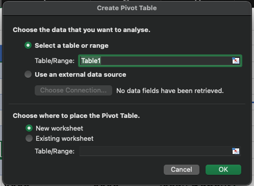
You’ll be prompted to choose the data you wish to analyse, and to provide a location for the Pivot Table. I usually have a worksheet tab dedicated to them, so they’re kept separate from the data they’re summarising.
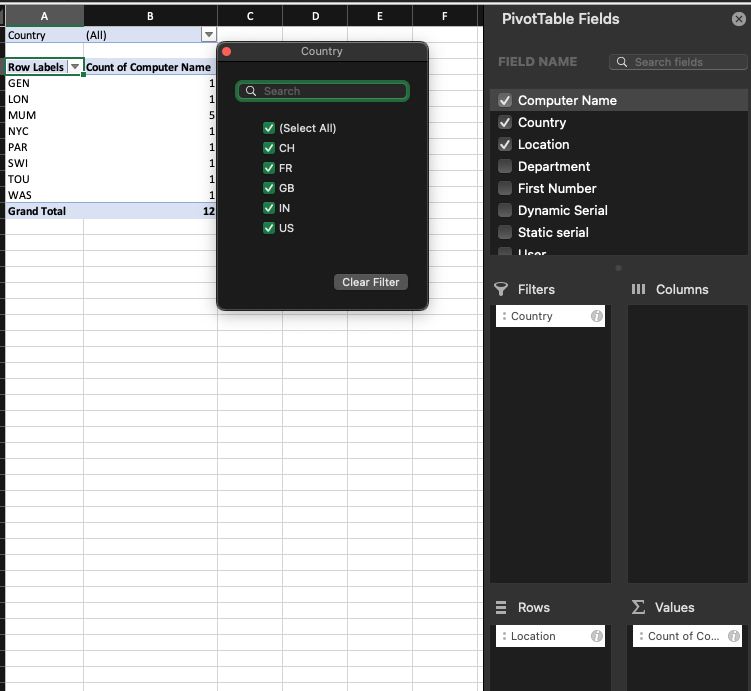
Once you’ve chosen a location, the Pivot Table placeholder is created and you can start to build it. At a minimum you need Rows and Values. Usually, you’ll only compute values from a single field, but it’s common to have multiple rows per value. For example, you might summarise computer counts by Country and Office Location. To do this, add Country and Office Location to Rows, & Computer Name to Values. Excel will likely automatically detect that Computer Name isn’t a number and will therefore use the Count function to count them.
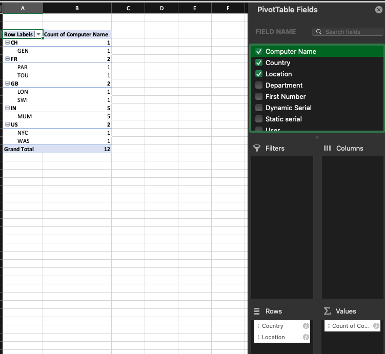
To take things a step further you can use Filters to restrict the data displayed in the pivot table. In the above example, moving Country from Rows to Filters provides a drop-down that enables summary of computers by Country.
This is just the tip of the pivot table iceberg, they’re incredibly powerful and useful tools. Importantly, remember that they’re non-destructive – they don’t change the underlying data – and so you can safely experiment with them.
However, there are some limitations, particularly around performance with large tables. Also, you can only work with data from a single table per pivot – which is why we looked at Index, Match, and XLOOKUP earlier so that we could combine data from multiple tables.
To move beyond those limitations, we need to look at how Microsoft have improved Excel with new tools including Power Pivot & Power Query.
Excel: The Next Generation
Microsoft recognised very early that much data analysis, dashboarding, and BI work takes place in Excel. There’s a whole cottage industry of Excel experts out there providing templates for dashboards, KPIs, and BI-like functions to try to match what you can get with Tableau, Qlik, and other solutions. Microsoft’s in-house answer to this use case is Power Pivot & Power Query, both of which are built-in to Windows versions of Excel and included with your Office license. To go even further there is the option to subscribe to Power BI for an additional monthly fee. The primary benefit of these new tools is that they bring even more rigour to the process of acquiring and transforming data from external sources. Most importantly, once you’ve built your query using Power Query and pivot tables in Power Pivot, all the inevitable legwork required to transform or normalise source data is done and is saved ready for use the next time you need to carry out data analysis.
If you have expertise in using Power Pivot & Power Query for ITAM tasks we’d love to hear from you, either in the comments or via email.
Summary
Excel has always been the go-to tool for ad hoc data wrangling. Its power, accessibility, and ubiquity mean that you can very quickly learn the basics and move on to advanced topics. And, with Microsoft adding Power Query & Power Pivot, you may well find that it’s all you need to produce rich, detailed, and accurate summaries of your ITAM data.
Acknowledgements
Thanks to everyone who responded to my question on LinkedIn and shared their expertise. If you’ve got something to add, please follow up in the comments. We’d particularly welcome a follow-up article looking at using Power BI, Power Query, and Power Pivot for common ITAM tasks. If you’re interested in contributing that please email support@itassetmanagement.net
Further Reading
Can’t find what you’re looking for?
More from ITAM News & Analysis
-
Flexera is first SAM tool vendor verified for Oracle E-Business Suite applications
Flexera has announced that it has been verified as the first software asset management (SAM) tool vendor for Oracle E-Business Suite applications. Almost anyone with an Oracle estate will be familiar with the company’s License Management ... -
ITAMantics - March 2024
Welcome to the March 2024 edition of ITAMantics, where George, Rich and Ryan discuss the month’s ITAM news. Up for discussion this month are. Listen to the full ITAMantics podcast above or queue it up from ... -
ITAM & AI, FinOps, Containers, ESG, security: The many ways in which ITAM has matured beyond its roots
ITAM, AI, FinOps, Containers, ESG, security… Back in January I wrote about my picks from the agenda for Wisdom NA 2024. Building up to the event I also interviewed Eva Louis about the intricacy of IT ...